Orion’s Sword
Click image for full size version
February 22, 2026
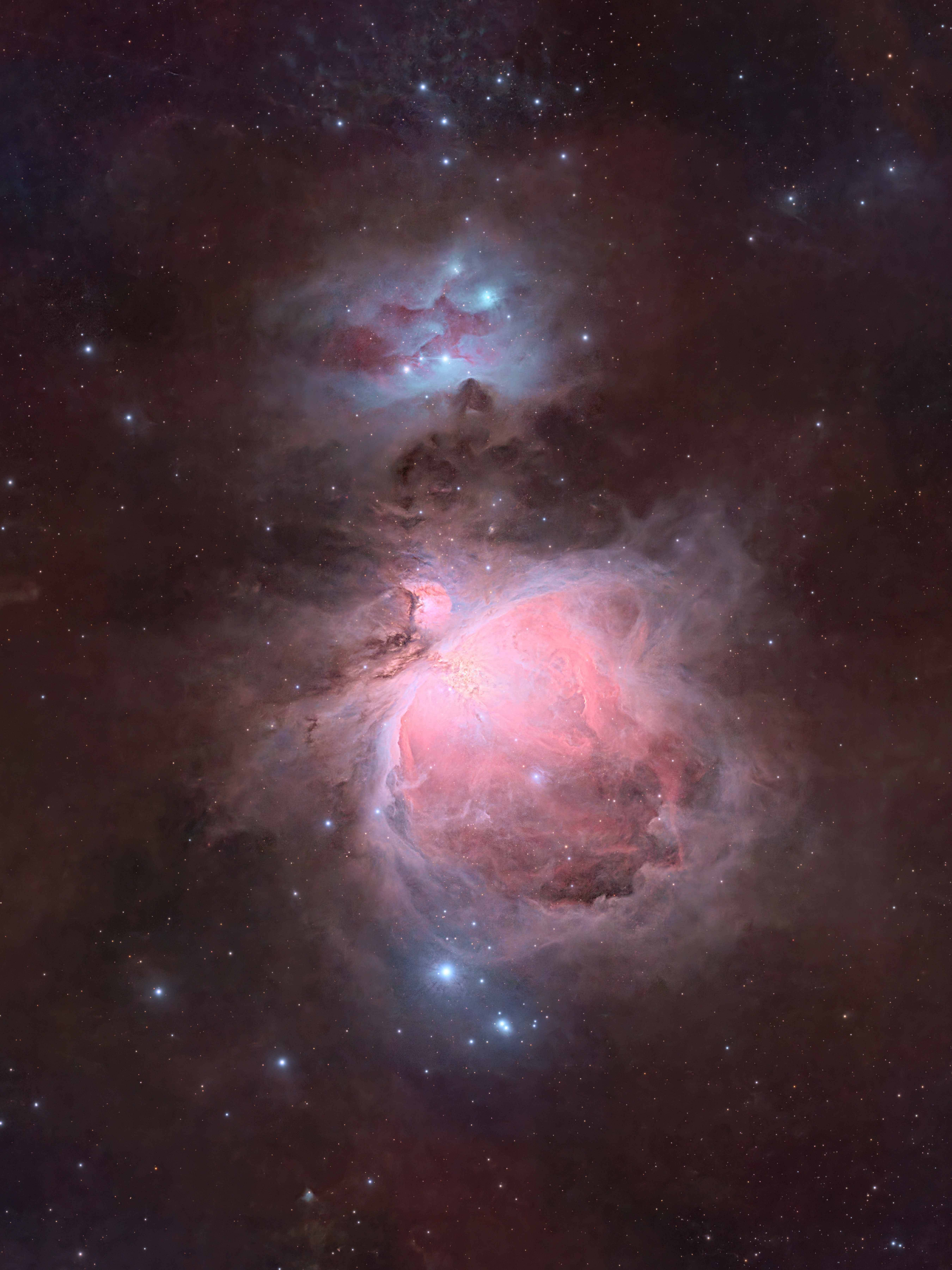
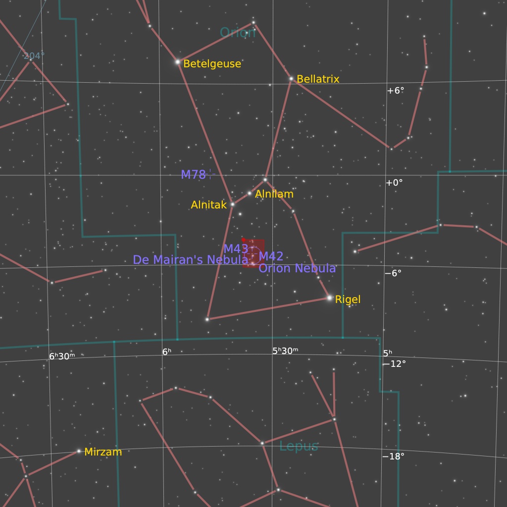
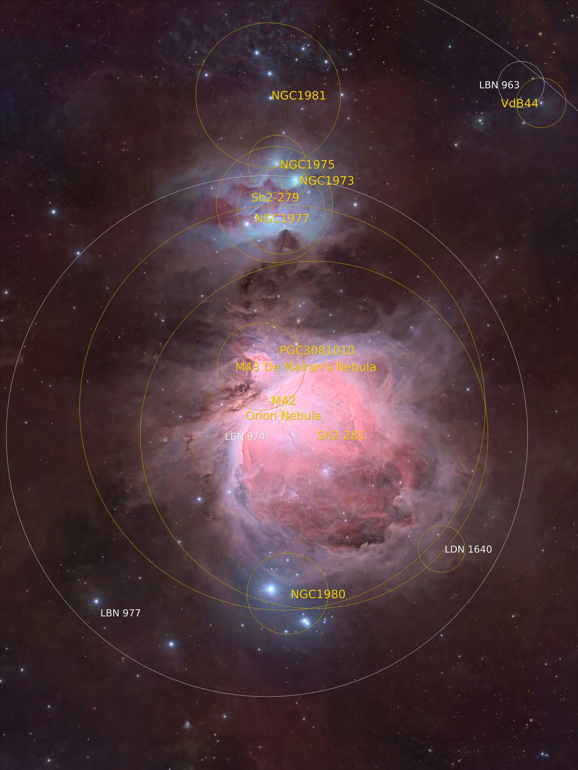
Orion’s Sword might be my favourite single star field in the sky, but I could probably say that about a dozen other objects. There’s a lot going on in this field. The largest object in the image is the Orion Nebula, also known as M42. Above it is the Running Man Nebula, NGC 1977. These objects contain both emission (reddish) and reflection (bluish) nebula components. There are also star clusters, and lots of interstellar dust and soot visible in this image. Together, this group of objects makes up Orion’s sword, which hangs from the hunter’s belt in the southern sky early in the evening at this time of year. If you look closely at the core of the Orion Nebula, you can see the quadruple star theta Orionis (known as “The Trapezium”) which is well resolved in this image. I also prepared an annotated image that identifies most of the deep-sky objects in this amazing field of view.
Tekkies:
Acquisition, focusing, and control of Paramount MX mount and other equipment with N.I.N.A. and TheSkyX. Unguided, Focus with Primalucelab Sesto Senso 2. Equipment control with Primalucelab Eagle 4 Pro computer. All pre-processing and processing in PixInsight. Acquired from my SkyShed in Guelph. Acquired under average transparency and seeing and no moonlight on February 14 and 17, 2025.
Sky-Watcher Esprit 70 EDX refractor, QHY367C Pro camera.
L-Quad Enhance Filter: 28 x 2m = 0hr 56m
41 x 1m = 0hr 41m
60 x 5s = 0hr 5m
Total: 1hr 42m
Preprocessing: The WeightedBatchPreProcessing script was used to perform calibration, cosmetic correction, weighting, registration, integration and Drizzle integration of all frames (2x drizzle, 1.0 Drop Shrink). Three masters were created from the 5s, 1m, and 2m individual frames.
HDR Image Creation:. HDRComposition was used with default settings to integrate the three masters into a single image that conserved core detail.
Gradient Removal: DynamicBackgroundExtraction was applied to the RGB master.
Colour Calibration: BlurXterminator was applied with Correct Only selected, followed by ColorCalibration.
Deconvolution: BlurXterminator was applied with Automatic psf , star sharpening set to 0.35, and non-stellar set to 0.9.
Linear Noise Reduction: NoiseXterminator was applied twith settings Amount=0.9 and Interations=4.
Stretching: MultiscaleAdaptiveStretch was applied to make a pleasing image. Approximate background level after stretch was 0.1.
Nonlinear Processing
Star Removal and processing: StarXterminator was used to remove the stars fwith Unscreen checked. Colour was increased in the RGB stars-only image by applying CurvesTransformation’s saturation through a star mask.
Nonlinear Noise Reduction: NoiseXterminator was applied to the image with settings Amount=0.9 and Iterations=5.
Contrast Enhancement: Jurgen Terpe’s MakeHDRImage was used to slightly compress the core of M42. LocalHistogramEqualization was then applied twice to the entire image without a mask. A Contrast Limit of 1.5 and 1 iteration was used for each application (scale 150, strength 0.35, and scale 40, strength 0.25).
Sharpening: With a mask to protect darker regions of the image, MultiscaleMedianTransform was used to sharpen Layers 1 – 5 with strengths of 0.02, 0.02, 0.01, and 0.01, respectively.
Star Restoration: Stars were added back into the image using the PixelMath expression combine(starless, stars_only, op_screen())
Final Steps: Background, galaxy, and star brightness, contrast, and saturation were adjusted in several iterations using CurvesTransformation and Jurgen Terpe’s SelectiveColorCorrection script with masks as required. ICCProfileTransformation (sRGB IEC61966-2.1; Relative Colorimetric with black point compensation) was applied prior to saving as a jpg. The finder chart was made using the FindingChart process. The annotated image was made with the AnnotateImage script.
Leave A Comment