NGC 6366
 Click image for full size version
June 13, 2026
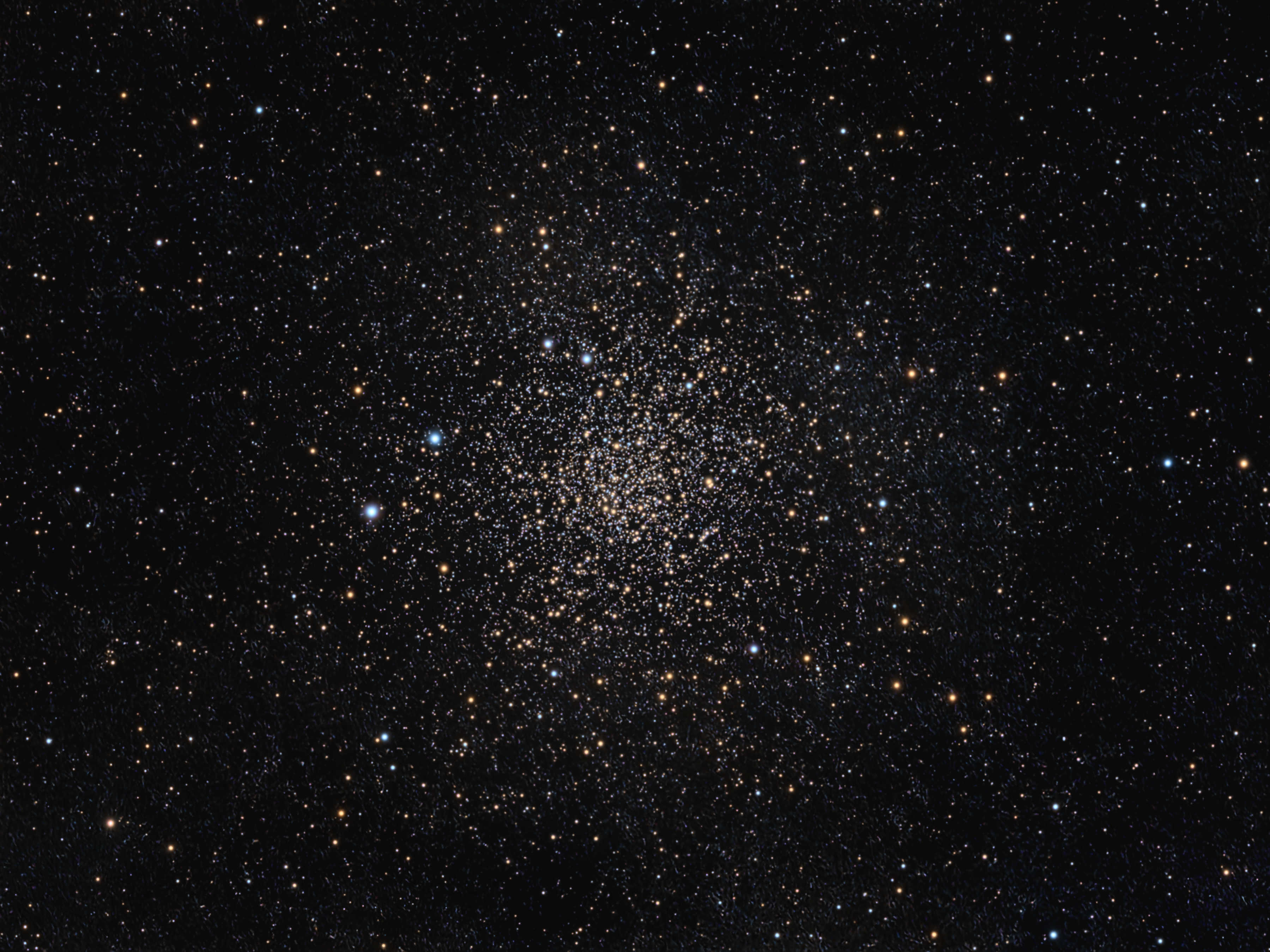
Meet NGC 6366, one of more than 150 globular clusters orbit the Milky Way’s core. Each is a more-or-less spherical grouping of hundreds of thousands of stars tightly held together by gravity. Some, like M13 are big, bright, tightly packed and spectacular. Others… not so much.
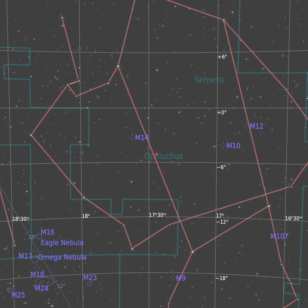
NGC 6366 is usually overlooked in favour of the splashier globular clusters of Ophiuchus, like M10, M12 and M14. It is so sparse that it barely looks like a globular cluster at all, except in long exposures like this one. It is small and dim (for a globular cluster), covering less than a half-Moon’s width in the sky. It lies 11,700 light years from us.
Although it might not compete with its siblings for brilliance, there are some facts that make it interesting: it is a “metal rich” cluster, meaning its stars have relatively large amounts of elements heavier than hydrogen and helium. It contains relatively few low mass stars; one theory is that the lower mass stars have been stripped away by the main portion of the Milky Way galaxy through “tidal stripping.”
I’ve imaged this object at least three times before, but this is the best so far, in my opinion. A previous version was published in the September 2015 Astronomy Magazine. Another image, from 2017, is posted here. Even my 2023 image doesn’t compare to the current version. It’s interesting to see how my equipment, processing workflow, and results have evolved over the last 11 or so years.
Tekkies:
Acquisition, focusing, and control of Paramount MX mount with N.I.N.A., TheSkyX. Primalucelab low-profile 2″ Essato focuser, ARCO rotator and Giotto flat panel. Guiding with PHD2 with QHY 585 guide camera. Equipment control with PrimaLuce Labs Eagle 4 Pro computer. All pre-processing and processing in PixInsight. Acquired from my SkyShed in Guelph. Average transparency and above average seeing. Acquired under moderate moon illumination from April 23-27, 2026.
Celestron 14″ EDGE HD telescope at f/11 (3,931 mm focal length) and QHY600M-SBFL camera binned 2×2 with Optolong filters.
18 x 5m Red = 1hr 30m
18 x 5m Green = 1hr 30m
18 x 5m Blue = 1hr 30m
Total: 4hr 30m
 .
. Preprocessing: The WeightedBatchPreProcessing script was used to perform calibration, cosmetic correction, weighting, registration, and integration.
RGB and SynthL masters: A master RGB image was made from the Red, Green and Blue Drizzled masters using ChannelCombination in RGB mode. A synthetic luminance (SynthL) master was made from all four masters using ImageIntegration with weighting by SNR.
Gradient Removal: DynamicBackgroundExtraction was applied to the SynthL and RGBmasters.
Colour Calibration: BlurXterminator was applied to the RGB master with Correct Only selected, followed by SpectrophotometricColorCalibration.
Deconvolution: BlurXterminator was applied to the RGB ane SynthL masters with Automatic psf, star sharpening set to 0.5, and non-stellar set to 0.9.
Linear Noise Reduction: NoiseXterminator was applied to the RGB and SynthL masters with settings Amount=0.9 and Interations=4.
Stretching: MultiscaleAdaptiveStretch was applied to make a pleasing image from the RGB and SynthL masters. Approximate background level after stretch was 0.09 for the RGB master ane 0.1 for the SynthL master.
Nonlinear Processing
Star Removal and processing: StarXterminator was used to remove the stars from the SynthLRGB master with Unscreen checked. Colour was increased in the stars-only image by increasing saturation using CurvesTransformation through a star mask.
Nonlinear Noise Reduction: NoiseXterminator was applied to the starless image with Amount=0.9 and Iterations=4.
Star Restoration: Stars were added back into the image using the PixelMath expression combine(starless, stars_only, op_screen())
Final Steps: Brightness, contrast, and saturation were adjusted in several iterations using HistogramTransformation and CurvesTransformation with masks as required. ICCProfileTransformation (sRGB IEC61966-2.1; Relative Colorimetric with black point compensation) was applied prior to saving as a jpg. The finder chart was made using the FindingChart process.
Nice work!!
Gorgeous image, of course!
Hi Ron, I’ve been an avid fan of your work for years. I did some film-based AP back in the day, and when COVID hit in 2020 I found myself with some time on my hands which I used to learn how to do digital AP. I’m still learning, of course, and have invested in equipment and software and have built up my skills quite a bit in the last few years. I’m still doing OSC, and will likely progress into mono at some point.
I have a question with respect to processing globular clusters specifically. I often run into what I call “the worms” – small, mostly linear artifacts which seem to be introduced (or made worse) in the NoiseXTerminator (linear) step. I’ve found that NxT AI version 2 doesn’t do this as badly as NxT AV version 3, but then again AI v2 doesn’t distinguish stars in the GC core as well as v3, either. Nothing I do has much of an effect on the worms, and they come out in both the stars and starless versions, and short of time-consuming Blemish Blasting (via SETI Astro), I can’t seem to not create them in the process.
Thoughts? Thanks – keep up the great work!
Hi Kevin. The core of a GC is a pretty high-signal region, and probably doesn’t need noise reduction. Consider using a mask that protects the core from NoiseXT. Hope this helps.